Example

The use of the above functions will be demonstrated with synthetic data provided above. After downloading the data files clean.mat and corrupted.mat in appropriate directory, these data can be loaded in MATLAB^TMworkspace:

>> load clean.mat; who 

Your variables are:

Signal

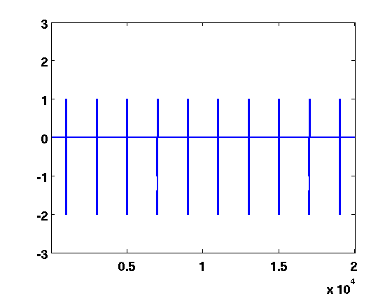
Your workspace now contains a variable Signal, which is a row vector of ``neural data'' to be analyzed. This data contains 10 equally spaced APs (transients). The attribute ``clean'' indicates that the data does not contain any noise. You can visualize the signal by:

>> plot(Signal)
>> set(gca,'XLim',[1 length(Signal)],'YLim',[-3 3])

Figure 1: Signal given in clean.mat plotted against time [samples].

The result is shown in Fig. 1. The sampling rate of the synthetic signal is 20 [kHz], and so Fig. 1 corresponds to 1 [s] of data. A close inspection of individual APs shows that they consist of two sinusoid semi-cycles of different amplitudes. The duration of the APs is set to 0.6 [msec]. The detection of APs in Signal is not very challenging, but reveals the true arrival times of APs:

>> TT = detect_spikes_wavelet(Signal,20,[0.5 1.0],6,'l',0.1,'bior1.5',1,1)
wavelet family: bior1.5
10 spikes found
elapsed time: 0.26422

TT =

  Columns 1 through 6

        1004        3004        5004        7004        9004       11004

  Columns 7 through 10

       13004       15004       17004       19004

The last two arguments in the function are plot and comment flags. To suppress comments and plots, you should pass a number different from 1, for example:

>> TT = detect_spikes_wavelet(Signal,20,[0.5 1.0],6,'l',0.1,'bior1.5',0,1);

produces comments but not plots, and

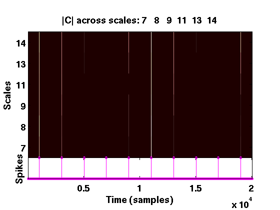
>> TT = detect_spikes_wavelet(Signal,20,[0.5 1.0],6,'l',0.1,'bior1.5',1,0);

produces plots but not comments. If you opt for plots, the script generates two figures: Fig. 2 and Fig. 3 (shown below).

Figure 2: Time-scale representation of the signal in clean.mat. The presence of strong coefficients at relevant scales coincides with the arrival times of APs.

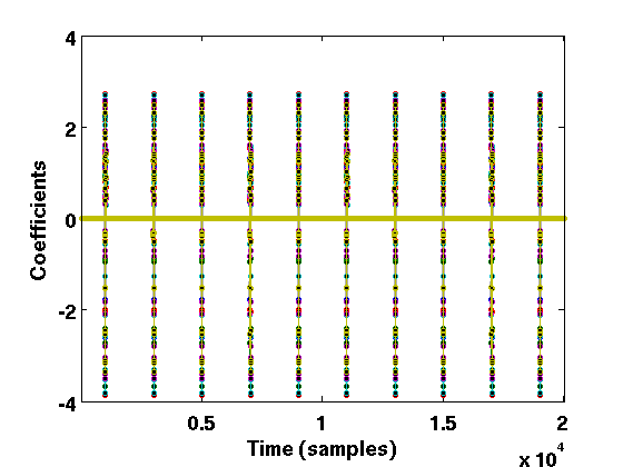
Fig. 2 shows the time-scale representation of the signal, where the absolute values of wavelet coefficients are color coded. At the bottom of the same plot are the locations (arrival times ) of the APs. By zooming in on this figure, it is obvious that the APs correspond to ``large'' coefficients across various scales.

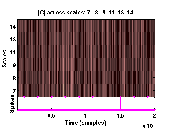
Fig. 3 shows the wavelet coefficients at different scales that cross the detection threshold. The coefficients at various scales are color-coded, e.g red, blue, green etc. The coefficients that do not cross the detection threshold are shrunk to 0.

Figure 3: The coefficients of the signal in clean.mat at relevant scales.

The 1st argument of detect_spikes_wavelet.m is the signal itself. The 2nd argument is the sampling rate of Signal in [kHz]. The 3rd argument is a vector that specifies the minimal and maximal duration in [ms] of APs to be detected. The 4th argument is the number of scales used in detection. In this case, 6 scales were used and they are roughly matched to APs lasting $\left\{\vphantom{0.5, 0.6, 0.7, 0.8, 0.9, 1.0}\right.$0.5, 0.6, 0.7, 0.8, 0.9, 1.0$\left.\vphantom{0.5, 0.6, 0.7, 0.8, 0.9, 1.0}\right\}$ [ms]. The 5th argument is an option l or c, referring to ``liberal'' and ``conservative'' mode of operation (see [2]). These two modes will produce similar results in most cases. Differences will arise in detection under extremely noisy conditions, where in the conservative mode the function will typically not return any detected APs, while in the liberal mode the function will most likely find APs of very small amplitude. The 6th argument is a sensitivity parameter, whose value typically ranges between -0.2 and 0.2. This parameter trades-off the cost of false alarm and omission. The higher the value of the parameter, the less likely the false alarms are and the more likely omissions are (see below). Finally, the 7th argument is the family of wavelet to use for detection. The wavelet from the family bior1.5 is used in this example.

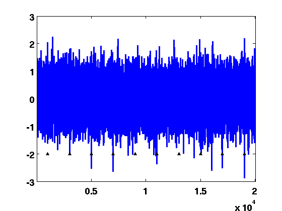
We now take the time series from above and corrupt it by adding a white noise, whose standard deviation determined from desired signal-to-noise ratio (SNR).

>> load corrupted.mat
>> plot(Signal)
>> set(gca,'XLim',[1 length(Signal)],'YLim',[-3 3])

By executing the code above, we can visualize the noisy neural data (see Fig. 4). Black arrows (plotted separately) indicate the arrival times of APs. Clearly, a simple detection based on amplitude thresholding could not detect low-amplitude APs (e.g. APs 1, 5 and 7) without accepting a number of false positives.

Figure 4: Signal given in corrupted.mat plotted against time [samples].

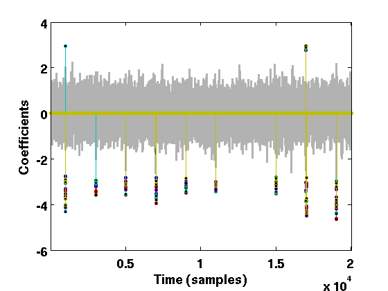
Then, we detect APs in the noisy data by

>> TE = detect_spikes_wavelet(Signal,20,[0.5 1.0],6,'l',0.1,'bior1.5',1,0);

which results in Figs. 5 and 6:

Figure 5: Time-scale representation of the signal in corrupted.mat. The presence of strong coefficients at relevant scales coincides with the arrival times of APs.

Figure 6: The coefficients of the signal in corrupted.mat at relevant scales.

As can be seen from the figure above, one of the spikes (spike 7) was not detected. This can be verified by running the function get_score.m which returns the number of correctly detected spikes, the number of omissions as well as the number of false positives. Indeed, running

>> get_score(TT,TE,20)

ans =

     9     1     0

indicates that there are 9 correctly detected spikes, 1 omission and 0 false positives. You can trade-off omissions and false positives by varying the parameter L (type help detect_spikes_wavelet to learn more about this parameter), i.e.

>> TE = detect_spikes_wavelet(Signal,20,[0.5 1.0],6,'l',0.05,'bior1.5',0,0);
>> get_score(TT,TE,20)

ans =

    10     0     3

indicating that all APs have been detected (no omissions). The paid price, however, is in the 3 false positives. You can now play with different choice of wavelet functions, such as 'bior1.3' 'db2' 'haar' etc., and compare their performances.