Example

Application of CPCA will be demonstrated on a simple letter recognition problem. Its role is to merely introduce the technique, though I increased the noise considerably to make the problem at least non-trivial. Assume that noisy images of letters I and K are provided, as shown in Fig. 1 and Fig. 2, respectively. You may or may not be able to recognize the letters, as the values of noise-free images range from 0 to 255, while the noise standard deviation is 1000. Thus, the signal-to-noise ratio is extremely low, as often seen in analysis of brain functional images.

Figure 1: 20 noisy images of letter I.

Figure 2: 20 noisy images of letter K.

To generate these images, the following files are needed:

1. generate_letter_samples.m
2. LI.mat
3. LK.mat

The letters matrices, I and K, can be generated by running

[I, K]=generate_letter_samples(20,20,1000,1000);

in MATLAB command prompt (presumably from the same directory where the above 3 files are stored). The respective dimensions of I and K are 111 x 81 x 20, indicating that there are 20 instances of letter I and 20 instances of letter K, as shown in Fig. 1 and Fig. 2, respectively. Note that the dimension of the data is 8991 ( 111 x 81), and that we have a severe small sample size problem. The second argument 1000 indicates the standard deviations associated with these images. To visualize a single image, you could run the following snippet:

colormap gray
imagesc(I(:,:,1))
set(gca,'DataAspectRatio',[1 1 1])

You may need to take an average over images to be able to visualize the letter, i.e. imagesc(mean(I,3)). To proceed, these 3D arrays are reshaped into 2D arrays (matrices). The following snippet will do the job for the matrix I:

IR = zeros(size(I,3),size(I,1)*size(I,2));
for i = 1:size(I,3)
IR(i,:) = reshape(I(:,:,i),1,size(I,1)*size(I,2));
end

Similar procedure can be applied to K. Note that the data is in the format n x N, where n is the number of trials (instances) and N = 8991 is the total dimension of the data. We concatenate this data into a single training data matrix: TrainData = [IR; KR];, and we form a vector of class labels: TrainLabels = [zeros(size(IR,1),1); ones(size(KR,1),1)]. We have therefore assigned labels 0 and 1 to letters I and K, respectively. We can now apply CPCA by running:

 DRmatC = dataproc_func_cpca(TrainData,TrainLabels,1,'empirical',{'mean'},'aida');

The first two input arguments are defined above. The third one is the dimension of the final space (we choose m = 1). The next argument describes the way prior (class) probabilities are estimated ('empirical' means that the class relative frequencies are preserved; in our example [0.5 0.5], since there are 20 instances of I and 20 instances of K). The next argument specifies the eigenvalues to be kept in the CPCA process ({'mean'} indicates that eigenvectors corresponding to the eigenvalues higher than the mean of nonzero eigenvalues are to be kept). Finally, the last argument specifies the type of data dimensionality reduction technique to be used ('aida' refers to the technique developed in [4], but a good old linear discriminant analysis (LDA) can also be used at this point). You can download both LDA and AIDA (together with its auxiliary functions) by following the links provided below. For more information, type help dataproc_func_cpca in MATLAB command prompt.

1. http://cbmspc.eng.uci.edu/SOFTWARE/CPCA/linear_disc_analysis.m
2. http://cbmspc.eng.uci.edu/SOFTWARE/AIDA/aida.html

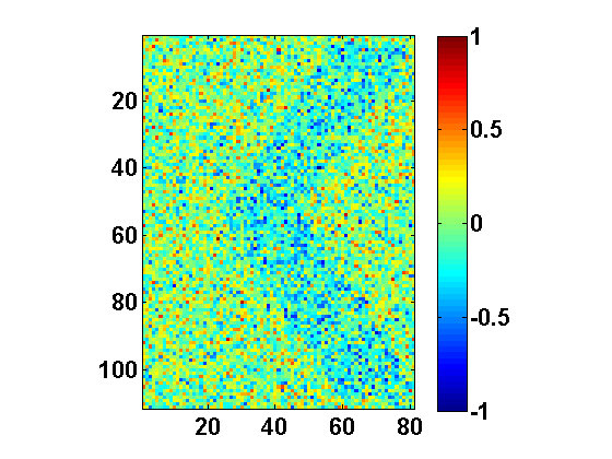
The function returns two 1D subspaces: DRmatC{1} and DRmatC{2}. These subspaces (one for each class) appear due to nonlinearity (piecewise linearity) of CPCA. Each subspace can be seen as feature extraction mapping from the original N-dimensional data space into 1D feature subspace. They also have a physical interpretation as they point to the areas of image (pixels) that encode the differences between I and K. In particular, reshaping these vectors back into the matrix form yields the image in Fig. 3. The following snippet will do the job for DRmatC{1} (roughly subspace corresponding to letter I):

colormap jet
M = max([abs(DRmatC{1}); abs(DRmatC{2})]);
imagesc(reshape(DRmatC{1},size(I,1),size(I,2))/M,[-1 1]); 
set(gca,'DataAspectRatio',[1 1 1])
colorbar

Similar code can be implemented to display DRmatC{2}. It can be noted that both subspaces feature a prominent < shape (Fig. 3), which essentially represents the difference between K and I.

Figure 3: (left) Subspace DRmatC{1} corresponding to letter I. (right) Subspace DRmatC{2} corresponding to letter K. The components of both subspaces have been normalized between -1 and +1. Dark colors (red or blue) imply important components, whereas those close to 0 are likely due to noise fluctuations.

You can visualize the (projection of) the training data onto the subspaces DRmatC{1} and DRmatC{2} by simply running:

subplot(121)
bh = plot(TrainData(TrainLabels==0,:)*DRmatC{1},1,'b*');
hold on
rh = plot(TrainData(TrainLabels==1,:)*DRmatC{1},1,'r*');
legend([bh(1),rh(1)],'class 0','class 1')
subplot(122)
bh = plot(TrainData(TrainLabels==0,:)*DRmatC{2},1,'b*');
hold on
rh = plot(TrainData(TrainLabels==1,:)*DRmatC{2},1,'r*');
legend([bh(1),rh(1)],'class 0','class 1')

To formally conclude the feature extraction process, one of the two subspaces above needs to be chosen given an unlabeled data point (image). This can be accomplished by calling the function choose_subspace.m. In particular, let us generate test data by calling:

[It, Kt] = generate_letter_samples(100,100,1000,1000); 

ItR = zeros(size(It,3),size(It,1)*size(It,2));
for i = 1:size(It,3)
    ItR(i,:) = reshape(It(:,:,i),1,size(It,1)*size(It,2));
end

KtR = zeros(size(Kt,3),size(Kt,1)*size(Kt,2));
for i = 1:size(Kt,3)
    KtR(i,:) = reshape(Kt(:,:,i),1,size(Kt,1)*size(Kt,2));
end

TestData =[ItR; KtR];
TestLabels = [zeros(size(ItR,1),1); ones(size(KtR,1),1)];

This snippet of code generates 100 test instances of I and K, reshapes them in the required format, and assigns their labels in the same manner it was done with the training data. To determine the optimal subspace for the first data point, we could run

[s,c] = choose_subspace(TestData(1,:),TrainData,TrainLabels,DRmatC,'empirical');

Again, you can type help choose_subspace to learn more about this function. Briefly, given a single instance of test data TestData(1,:), we decide on its optimal subspace for representation and presumably future classification. The output s gives the label of the optimal subspace for this test sample, and so the corresponding optimal subspace is DRmatC{s}. The label takes values from 1 to C, where C is the number of classes (subspaces). Once the subspace is known, the test sample as well as the training data can be projected onto the subspace, and classification can be performed. The following code will perform this operation on 200 test samples:

for i = 1:size(TestData,1)
    [s,c] = choose_subspace(TestData(i,:),TrainData,TrainLabels,DRmatC,'empirical');
    S(i) = s;
    Subspace{i} = DRmatC{s};
end

for i = 1:size(Subspace,2)
    ind = find(S == i);
    TestFeatures = TestData(ind,:) * Subspace{i};
    TrainFeatures = TrainData * Subspace{i};
    CL(ind) = classify(TestFeatures,TrainFeatures,TrainLabels,'linear','empirical');
end

The top loop finds the optimal representation subspace for each test sample. The bottom loop projects each test data onto its optimal subspace and trains a linear Bayesian classifier in this subspace. The variable CL contains the predicted labels of TestData. The function classify is a built-in MATLAB function that implements the Bayesian classifier. By calculating the confusion matrix (see Table 1)

Table 1: Confusion matrix. Rows are true identities of test images, while columns are their predicted identities. Performance based on 200 samples (100 per each letter class).

	I		K
I	1.0000		0
K	0.0300		0.9700

we see that I is predicted correctly 100% of the time, while K is misclassified as I in 3% of the cases and correctly classified in 97% of the cases. Here is the snippet that will generate the confusion matrix (your results may be slightly different due to randomization):

classes = unique(TrainLabels);
Nclass = length(classes);
for i = 1:Nclass
    %true state
    indc = find(TestLabels == classes(i));
    for j = 1:Nclass
        P(i,j) = sum(CL(indc) == classes(j))/length(indc);
        Sub(i,j) = sum(S(indc) == j);
    end
end
sprintf('[%1.2f  %1.2f]\n',P)

Let us conclude with few remarks:

• The final subspace dimension m need not be 1.
• The method can handle more than 2 classes.
• If the training data is unbalanced (significantly more samples in one class than the other), keeping things at m = 1, choosing lower number of eigenvalues to keep (e.g. use 'spectrum' or {'energy', xx}, where xx is a sufficiently low number), and using the linear Bayesian classifier, typically keep things under control. Additionally, using information discriminant analysis:
  • http://cbmspc.eng.uci.edu/SOFTWARE/IDA/ida.html
  for feature extraction may boost the performance. Type help dataproc_func_cpca for further info.

For details and limitations of the technique, please refer to [1].